TinyML Speech Recognition for Smart Home Assistant, Part 1
After reading one of my 2019 favourite books, ‘TinyML: Machine Learning with TensorFlow Lite on Arduino and Ultra-Low-Power Microcontrollers’ by Daniel Situnayake and Pete Warden. I decided to build a TinyML project for my final Capstone at Institute of Data, where I later got hired to the Data Science Training Team instantly after presenting the Speech Recognition project. In this post, I’ll introduce the concept of TinyML, why it is a giant opportunity as well as sharing step-by-step guide to build yourself a personal TinyML Speech Recognition Virtual Assistant.
1. What is TinyML?
The ‘Tiny’ here mentions about the Ultra-Low-Power microcontrollers and ‘ML’ simply stands for Machine Learning. As a combination, TinyML is an emerging concept to run Machine Learning inference with TensorFlow Lite on the Ultra Low-Power microcontrollers such as: Arduino, Sparkfun Edge and STMicroelectronics boards.
This ideal is developed by the OK Google team initially in 2014. They were running a 14 kilobytes (KB) deep neural networks on the digital signal processors (DSPs) present in most Android phones, which continuously listening for the “OK Google” wake words. In addition, these DSPs had only tens of kilobytes of RAM and flash memory; and these specialized chips use only a few milliwatts (mW) of power. The purpose of TinyML is for software and hardware developers who want to build embedded systems using machine learning and never worry about memory, battery or operating speed.
2. Why TinyML is the future?
Tiny Computers are Already Cheap and Energy Efficiency
Microcontrollers (or MCUs) are packages containing a small CPU with possibly just a few kilobytes of RAM, and are embedded in consumer, medical, automotive and industrial devices. They are designed to use very small amounts of energy, and to be cheap enough to include in almost any object that’s sold, with average prices expected to dip below 50 cents this year. The biggest benefit for the manufacturer is that standard controllers can be programmed with software rather than requiring custom electronics for each task, so they make the manufacturing process cheaper and easier. A microcontroller itself might only use a milliwatt or even less, a coin battery might have 2,500 Joules of energy to offer, so even something drawing at one milliwatt will only last about a month. Of course most current products use duty cycling and sleeping to avoid being constantly on, but you can see what a tight budget there is even then.
Deep Learning Runs Well on Existing MCUs
Microcontrollers (MCUs) tend to be less expensive than, simpler to set-up, and simpler to operate than microprocessors (MPUs). The comparatively low memory requirements (just tens or hundreds of kilobytes) also mean that lower-power SRAM or flash can be used for storage. This makes deep learning applications well-suited for microcontrollers, especially when eight-bit calculations are used instead of float, since MCUs often already have DSP-like instructions that are a good fit. This idea isn’t particularly new, both Apple and Google run always-on networks for voice recognition on these kind of chips, but not many people in either the ML or embedded world seem to realize how well deep learning and MCUs match.
TinyML Makes Sense of Sensor Data
In the last few years its suddenly become possible to take noisy signals like images, audio, or accelerometers and extract meaning from them, by using neural networks. Because we can run these networks on microcontrollers, and sensors themselves use little power, it becomes possible to interpret much more of the sensor data we’re currently ignoring. For example, every morning an engineer needs to walk along the row of machines to check which will have to be taken offline for servicing. If every machine could be attached a battery-powered accelerometer and microphone that would learn usual operation and signal if there was an anomaly, you might be able to catch issues before they became real problems. There are probably a hundred products I could dream up, but running neural networks on voice recognition is the main project I’d like to explain details in this post. Let’s get it started!
3. Building TinyML Speech Recognition.
In the TinyML book, Peter Warden covers about the Tensorflow Lite conversion and deployment of Speech Recognition model on different microcontroller chips (source code can be found on Tensorflow Github page). However, before deployment, the detail instructions of data extraction, data analytics and model building aren’t listed there. Hence, the steps below will fully cover from extracting .wav files data to deploying neural networks on an Arduino board. (code can be found on my Github page)
Materials:
- A laptop with Windows/ Mac/ Linux/ Ubuntu operating system.
- An Arduino BLE board
- Micro USB cable
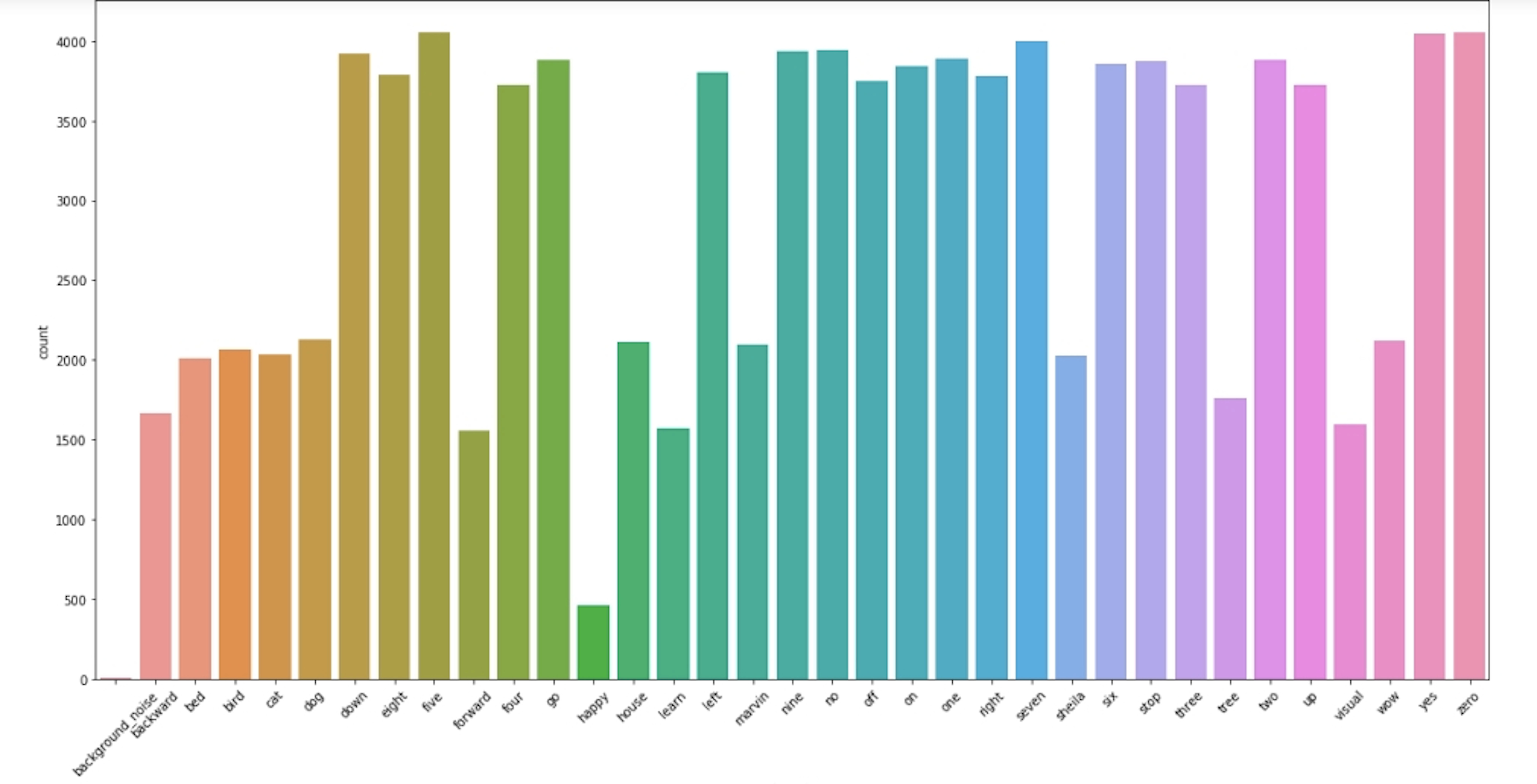
The audio files are collected from a research project of Google TensorFlow named ‘Simple Audio Recognition’. In detail, the archive Speech Commands data set is over 2GB and contains 36 different key words in 108,000 WAVE audio files in the list below:
‘four’, ‘forward’, ‘off’, ‘five’, ‘on’, ‘six’, ‘down’, “house’, ‘two’, ‘visual’, ‘up’, ‘zero’, ‘three’, ‘stop’,’follow’, “happy’, ‘backward’, ‘learn’, ‘cat’, ‘right’, ‘eight’, ‘sheila’, ‘nine’, ‘yes’, ‘one’, ‘no’, ‘left’,’tree’, ‘bed’, ‘bird, ‘go’, ‘wow’, ‘seven’, ‘marvin’, ‘dog’, “background_noise’.
This data was collected by Google and released under a CC BY license, and you can help improve it by contributing five minutes of your own voice at the on-going Open Speech Recording project. The audio file is mainly selected to be clear and clean for training purposes, therefore audio noises has been reduced or eliminated.
Step 1: Download and Extract
Download the speech-commands data set from here.
Extract tar.gz file
import tarfile
tar = tarfile.open('.../data_speech_commands_v0.02.tar.gz', "r:gz")
tar.extractall(path='extracting_folder_path')
tar.close()
Step 2: Data Analytics and Visualisation
After setting up a data pipeline to load all ‘.wav’ files, I built a function to choose randomly an audio for data analysing and visualising purposes. (You can find the project code on my Github page.)
In this case, ‘two’ is randomly chosen. Let’s quickly listen to it!
What you have just heard is a sound of 16 000 Hz frequencies. According to the Official Frequency Chart, the “perfect” human ear can hear frequencies ranging from 20Hz to 20 000 Hz. In addition, nowadays most music’s frequencies can be found around 50Hz and 16 000 Hz; and the visualisations below show the Digital Signal Processing (DSP) of ‘Two’ in various forms.
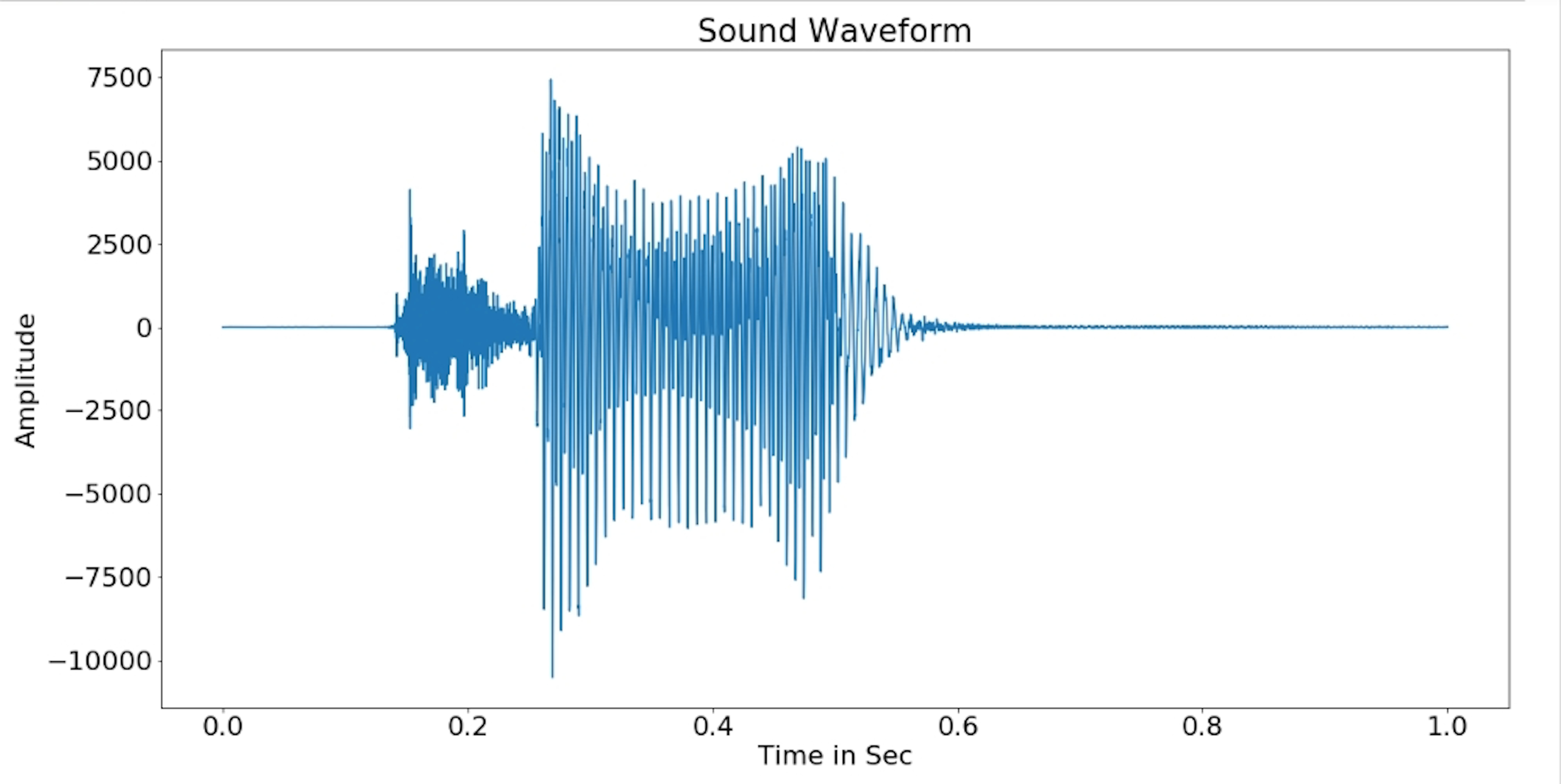
Sound Wave Form: This is the most common digital signal form, whenever a song is played; the screen on your device will automatically show the audio sound wave’s amplitude varies through time.
from scipy.io import wavfile
import pandas as pd
import numpy as np
import matplotlib.pyplot as plt
path = 'audio_file'
fs, signals = wavfile.read(path)
def plot_sine_wav(file_path):
    time = np.linspace(0, len(signals)/fs, num=len(signals))
    plt.plot(time,signals)
    plt.xlabel('Time in Sec')
    plt.ylabel('Amplitude')
    plt.title('Sound Waveform')
    plt.show()
plot_sine_wav(path)
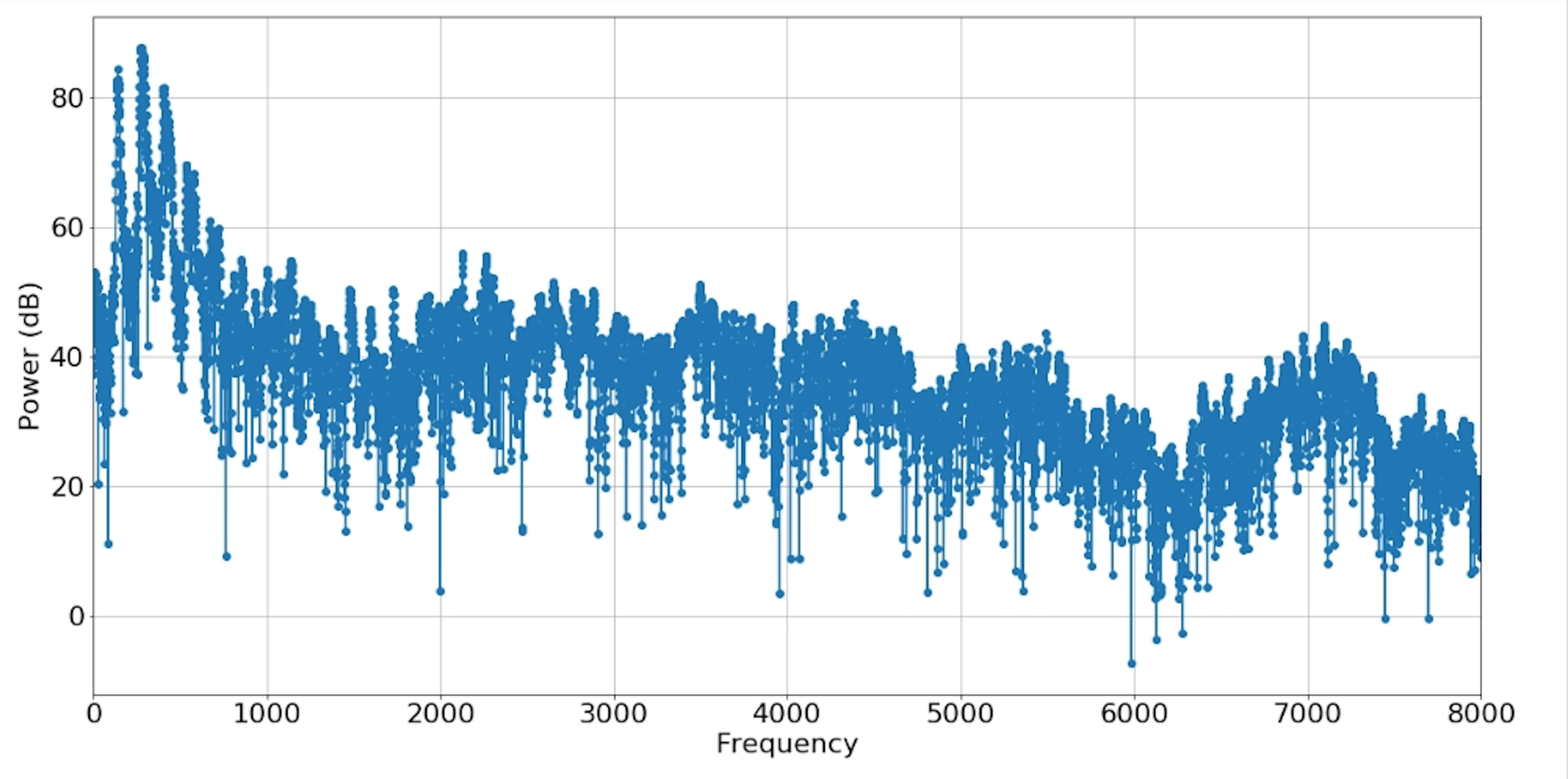
Periodogram Power Spectrum: describes the distribution of power into frequency components composing that signal. In signal processing, a periodogram is an estimate of the spectral density of a signal. One purpose of estimating the spectral density is to detect any periodicities in the data, by observing peaks at the frequencies corresponding to these periodicities.
from spectrum import Periodogram
plt.figure(figsize=(20,10))
plt.rcParams.update({'font.size': 22})
p = Periodogram(signals, fs)
p()
p.plot(marker='o')
Power Spectral Density: The power spectrum of a time serie describes the distribution of power into frequency components composing that signal.
from scipy import signal
f, Pxx_spec = signal.welch(signals, fs, 'flattop', 1024, scaling='spectrum')
plt.figure(figsize=(20,10))
plt.rcParams.update({'font.size': 22})
plt.semilogy(f, np.sqrt(Pxx_spec))
plt.xlabel('Frequency [Hz]')
plt.ylabel('Power [V RMS]')
plt.title('Power Spectral Density')
plt.show()
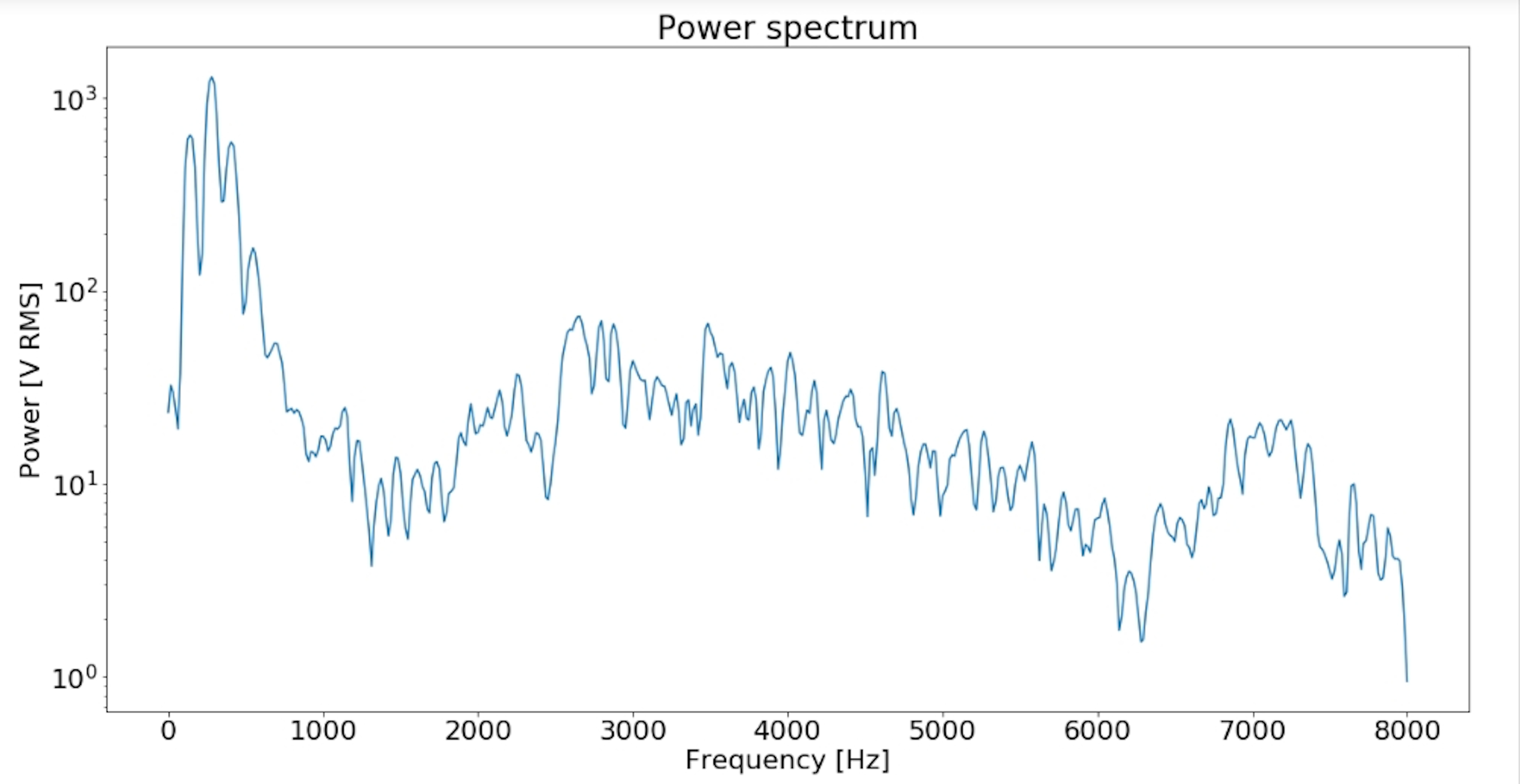
Fast Fourier Transform: The “Fast Fourier Transform” (FFT) is an important measurement method in the science of audio and acoustics measurement. It converts the signal of ‘two’ into individual spectral components and thereby provides frequency information about the signal. FFT is an optimized algorithm for the implementation of the “Discrete Fourier Transformation” (DFT). A signal is sampled over a period of time and divided into its frequency components. These components are single sinusoidal oscillations at distinct frequencies each with their own amplitude and phase.
def custom_fft(y, fs):
    T = 1.0 / fs
    N = y.shape[0]
    yf = fft(y)
    xf = np.linspace(0.0, 1.0/(2.0*T), N//2)
    vals = 2.0/N * np.abs(yf[0:N//2])
    return xf, vals
xf, vals = custom_fft(signals, fs)
plt.figure(figsize=(20,10))
plt.rcParams.update({'font.size': 22})
plt.title('FFT of speaker of ' +'Two')
plt.plot(xf, vals)
plt.xlabel('Frequency [Hz]')
plt.grid()
plt.show()
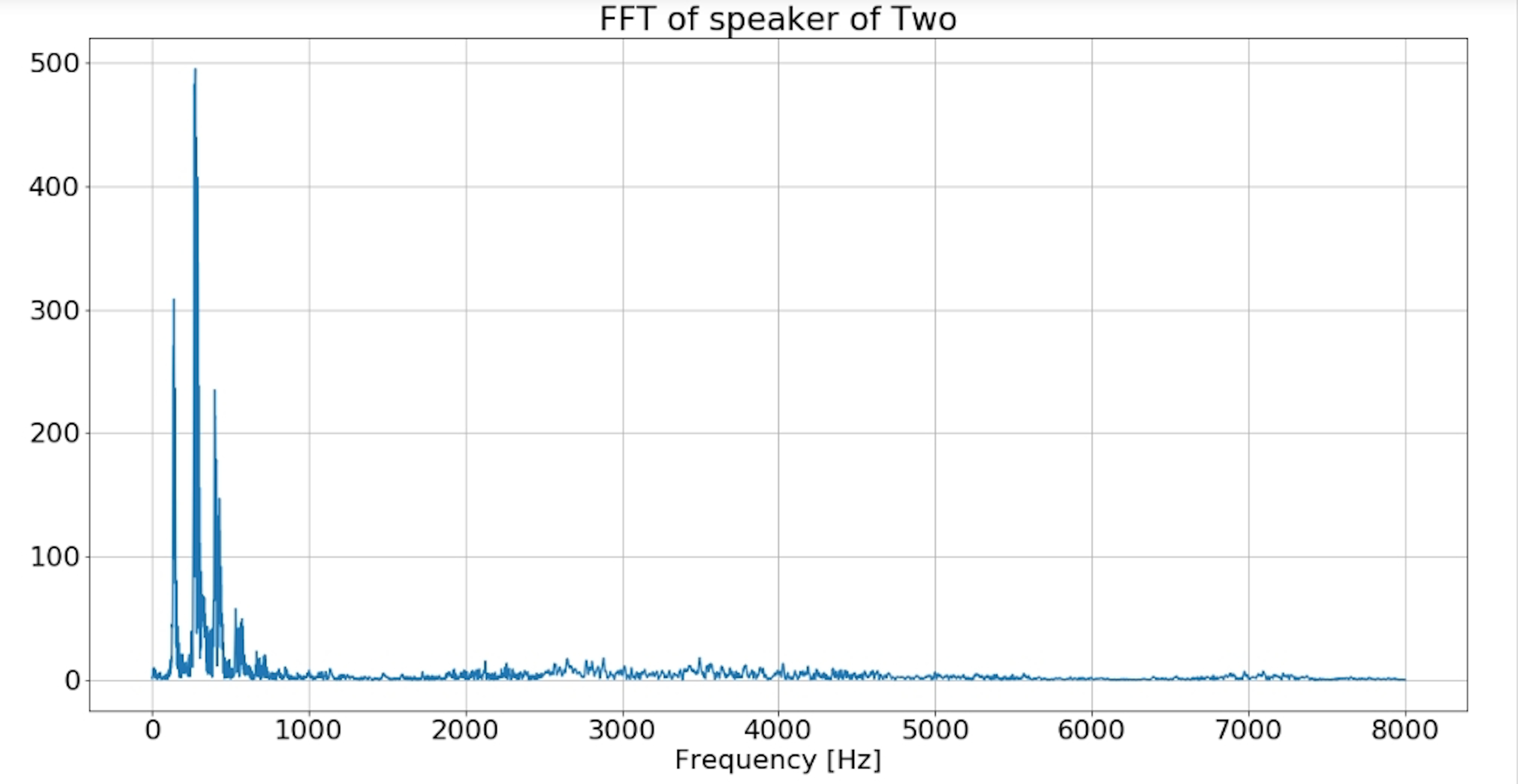
Spectrogram: is a visual representation of the spectrum of frequencies of a signal as it varies with time. When applied to an audio signal of ‘two’. In addition, spectrograms are sometimes called sonographs, voiceprints, or voicegrams.
def log_specgram(audio, sample_rate, window_size=20,
                 step_size=10, eps=1e-10):
    nperseg = int(round(window_size * fs / 1e3))
    noverlap = int(round(step_size * fs / 1e3))
    freqs, times, spec = signal.spectrogram(audio,
                                    fs=fs,
                                    window='hann',
                                    nperseg=nperseg,
                                    noverlap=noverlap,
                                    detrend=False)
    return freqs, times, np.log(spec.T.astype(np.float32) + eps)
freqs, times, spectrogram = log_specgram(signals, fs)

fig = plt.figure(figsize=(20,10))
plt.rcParams.update({'font.size': 19})
ax1 = fig.add_subplot(211)
ax1.set_title('Raw wave of '+'Two')
ax1.set_ylabel('Amplitude')
ax1.plot(np.linspace(0, fs/len(signals), fs), signals)

ax2 = fig.add_subplot(212)
ax2.imshow(spectrogram.T, aspect='auto', origin='lower',
           extent=[times.min(), times.max(), freqs.min(), freqs.max()])
ax2.set_yticks(freqs[::16])
ax2.set_xticks(times[::16])
ax2.set_title('Spectrogram of '+'two')
ax2.set_ylabel('Freqs in Hz')
ax2.set_xlabel('Seconds')

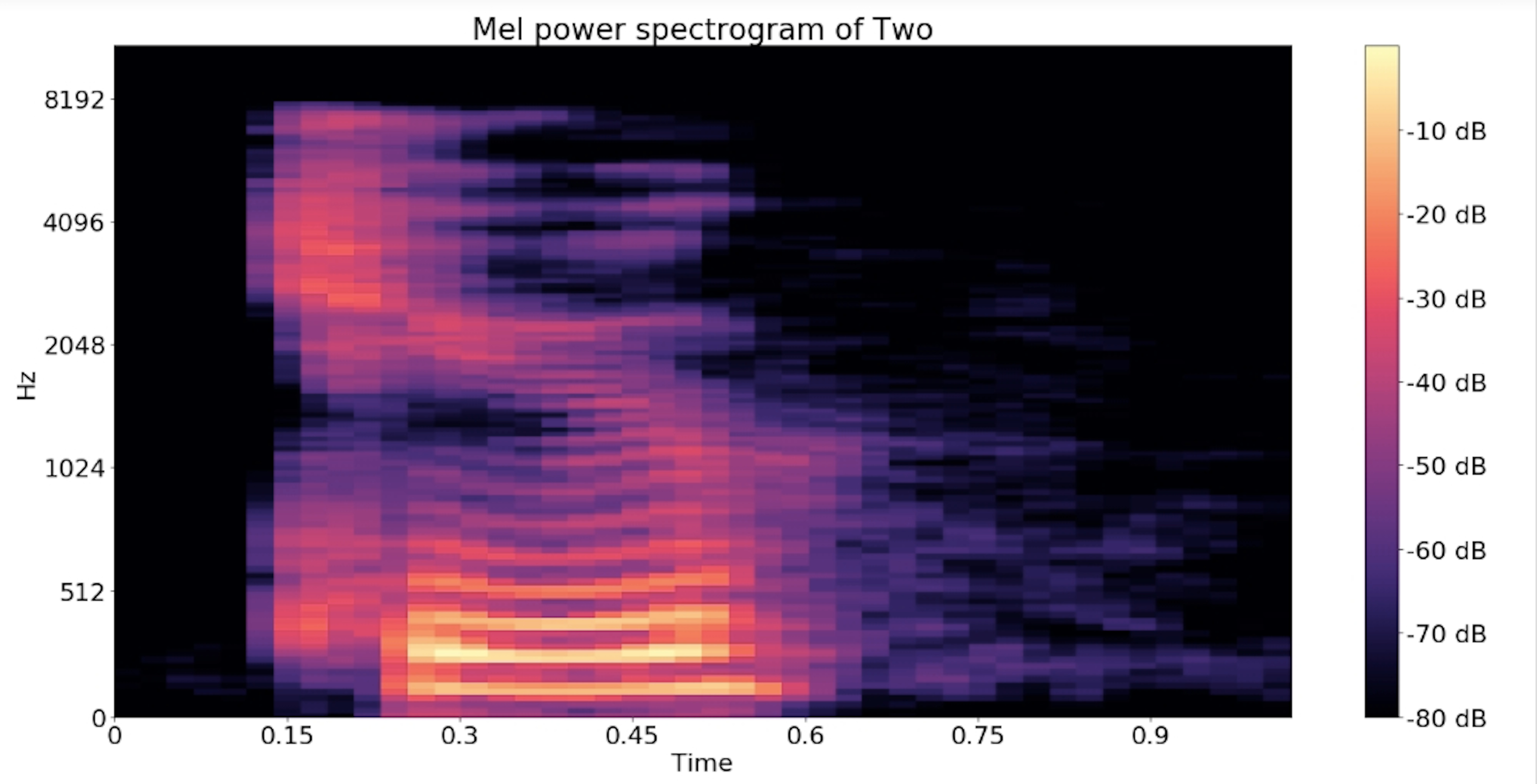
Mel-frequency cepstrum Spectrogram: is a representation of the short-term power spectrum of ‘two’, based on a linear cosine transform of a log power spectrum on a nonlinear mel scale of frequency.
import librosa
import librosa.display
y, sr = librosa.load(path)
S = librosa.feature.melspectrogram(y, sr=sr, n_mels=128)
# Convert to log scale (dB). We'll use the peak power (max) as reference.
log_S = librosa.power_to_db(S, ref=np.max)
plt.figure(figsize=(20,10))
plt.rcParams.update({'font.size': 22})
librosa.display.specshow(log_S, sr=sr, x_axis='time', y_axis='mel')
plt.title('Mel power spectrogram of '+'Two')
plt.colorbar(format='%+02.0f dB')
plt.tight_layout()
[To Be Continued…]
